EXAMPLE PROJECTS:
Our projects have covered a range of problems for both government and commercial clients. Here are a few examples.
Industry: Printing
Solution: Mathematical Modeling
Our client, a Fortune-20 company, wanted to create a cost-saving service for its clients in the printing industry. We used mathematical modeling to meet their requirements.
The service was designed to determine what fraction of a print job, such as an advertisement or product label for a mass-market consumer item, had subtle shadings of color. It would then decide whether to route the job automatically to an expensive printer that would be needed for the shading or to a less expensive one that would be adequate for anything else.
We defined and implemented the algorithms in MATLAB® application software, using fuzzy logic to model the eye’s perception and the brain’s judgment of well printed shading. The result over-performed the company’s expectations, even identifying important subtleties of shading that they had believed no algorithm could detect.
Industry: Software Development
Solution: Optimization and Caching
One of our clients was developing a MATLAB application for production use. However, it was running so slowly that even their software development and testing was impeded. The MATLAB Profiler showed that the problem was the reading of several huge arrays from disk, with total storage much larger than even virtual memory could accommodate. As a result, the app needed to read each array (slowly) into memory, use it once, and then discard it to free the memory again although each array was needed more than once even in a production run, and typically many more times during a develop-and-test cycle. Worse, for more complex cases, the app would exhaust memory and could not run at all.
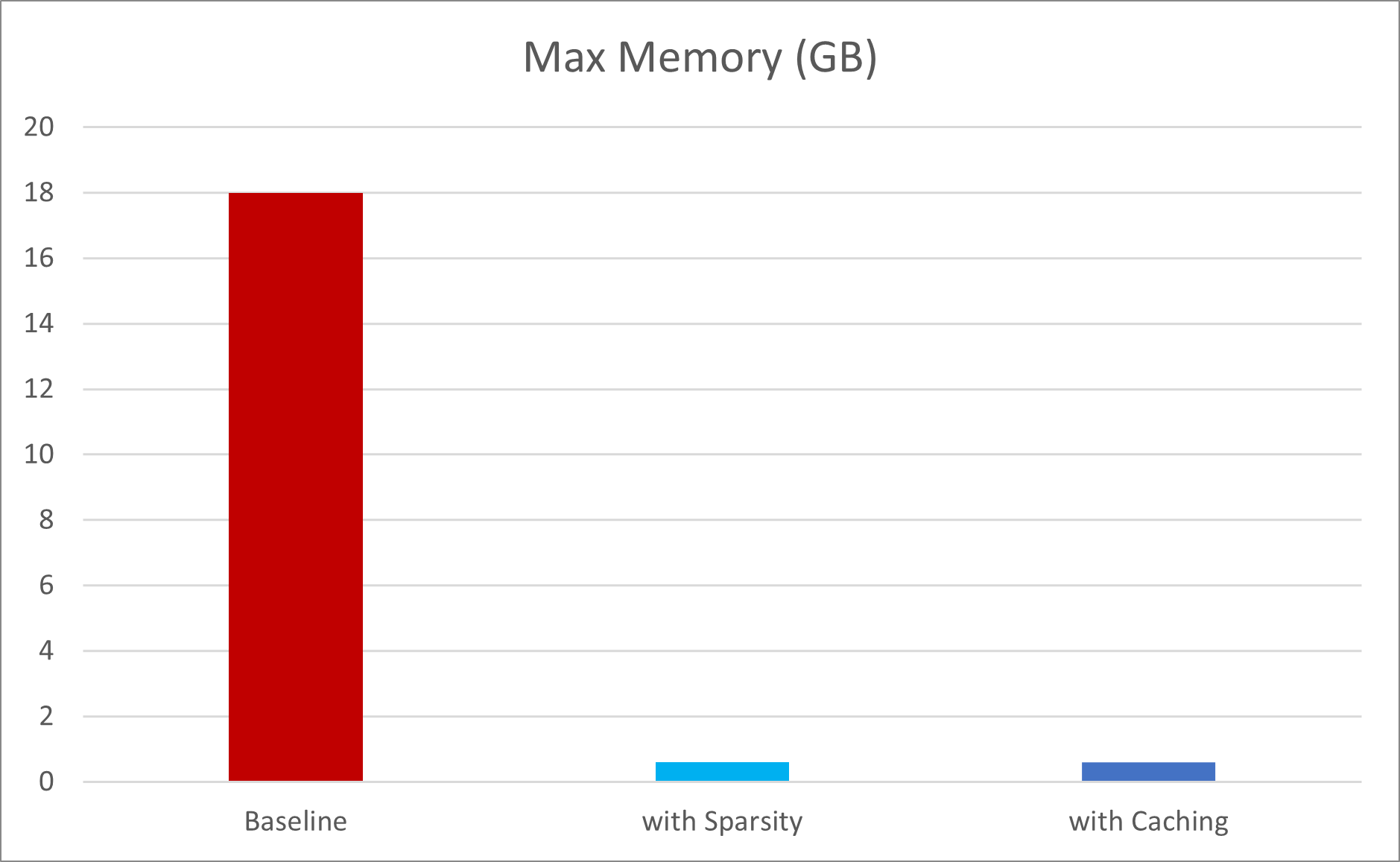 Our solution took two steps. A little sleuthing showed that, as stored on disk, the arrays were actually much smaller than when they were read into memory. The client confirmed that they were largely filled with zeros 97% or more. In fact, the arrays for more complex cases consisted of 99% zeros. So, our first step was to store them as MATLAB’s “sparse” arrays when in memory, a change to just two lines of existing code. Although reading them was no faster (in fact, a little slower to convert to sparse storage), many of them could now remain in memory during a run. Immediately, the app could handle more complex cases, and running time was cut in half.
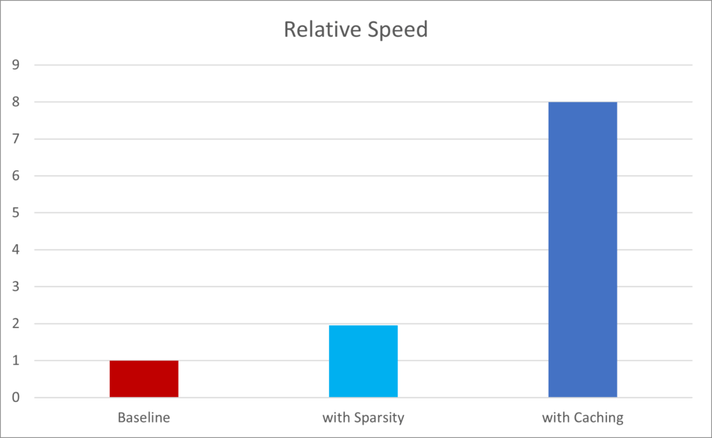 In the second step, we implemented a cache for the sparse arrays. With small changes to the same two lines of code, the caching function would always provide the arrays in their stored form, whether that entailed fetching from memory (if already stored there) or reading and storing first (if not).
The result was that, in practice, the app now ran 800% faster, and on a larger range of cases, greatly improving production use and removing a severe bottleneck in development.
Industry: Government
Solution: Optics and Image Processing
When fingerprints are classified, analysts use both the overall loop pattern of the skin’s ridges and “minutiae”, the specific locations where the ridges either split in two or end. With enough computing power, the minutiae alone can be very useful for automatically matching a scanned image of an individual’s fingerprint against a database of prints. This is the basis of AFIS, the FBI’s well known identification system.
But there are problems, as a government customer explained: When the finger receives a cut, this produces a large number of new “endings”, minutiae that cannot match any previous print, and may not even match future ones if the cut heals without scarring. Creases do the same. This is especially true in heavy manual labor (such as housecleaning!), which produces so many breaks that the sheer number of apparent minutiae might match practically anything. Also, if there are any stray marks on the image, stray materials on the finger, or fabric patterns underlying the print, these can falsely introduce or eliminate large numbers of minutiae.
We noted, however, that all the new endings occur in matched pairs, and all of the other defects introduce patterns that do not resemble the strong patterns of fingerprint ridges. This allowed us to devise algorithms to remove the new endings from the images, “rejoining” the cut ridges and suppressing the defect patterns. The result is an image of the print in a more pristine form: with just the ridges of the finger, splitting or ending just where they originally did on the finger. No cuts, no marks, no materials, no fabric!
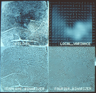
- a smudged area with poorly defined ridges near the top, from dirt and oil on the fingertip;
- a dark region of very little detail near the center;
- a large crease on the left, just below the center, as well as other creases.
Upper right: For each small section of the image, the processing identifies both the dominant local direction of ridge-like features, and the degree of contrast (variance, shown as brightness) between the ridges and valleys.
Lower left: The first cleanup: The process discards all details that are either too fine or too coarse to be ridges, regardless of direction. Then it identifies which pixels (picture cells) are brighter or darker than the local average by an amount equal to the contrast shown in the upper right image. Other pixels are assigned an intermediate shade of grey. (Despite the label, the image is not binary, i.e., not only black and white.)
Lower right: The second cleanup: Features that do not agree with the local direction (upper right image) — for example, creases, cuts, and even handwriting (not shown) — are now discarded. Most of the creases here are removed, with only faint ripples to show where they used to be.
The focus of processing is on clarifying the overall structure: a loop in the case, with its center slightly below and to the left of the image’s center. However, the result also yields well determined minutiae, places where a ridge ends or splits, over a much larger part of the fingertip, with very few false “ends” where a crease separates each ridge into two pieces. The processing here occurs independently in each small region, so even a very partial fingerprint can be processed, and minutiae revealed. The result is an image that is far easier to process for automated classification and analysis.
Industry: Speech Assessment
Solution: Knowledge-Based Machine Learning in an Expert System
For one government project in health services, we needed to develop a short but robust test to assess how well a non-native nurse or other speaker of English would be understood in English by a native “standard listener” (whether a human patient or … well, Amazon Echo!). The test had to be brief. It had to be automated and objective. Most of all, it had to be empirically validated with non-familiar human ears listening to conversation from the same speaker: the real world.
We began with an expert’s judgment for certain items: specific words and sentences in English, totaling no more than a few minutes to record. We compared speakers saying those items with listeners’ judgments of understandability after hearing a full minute of English conversation from them.
The expert’s judgment allowed us to process the specific words using fuzzy-logic algorithms of robust, knowledge-based speech processing: our SpeechMark® system based on the physics and physiology of speech. That gave us automatically computed features such as vowel duration and syllable count.
We implemented a classifier for each item, using soft-margin support-vector machines, training on those items as spoken by native speakers of English, Chinese, and Spanish — what linguists call the “L1” language of each speaker. In other words, for each item, we could score its pronunciation by how closely, and on which computed features, it matched native English speech.
The expert specified an architecture for combining the computed scores from individual items into a robust overall score for all the speakers. Then we trained the system to match the overall scores to the listeners’ understandability judgments for conversation from the same speakers.
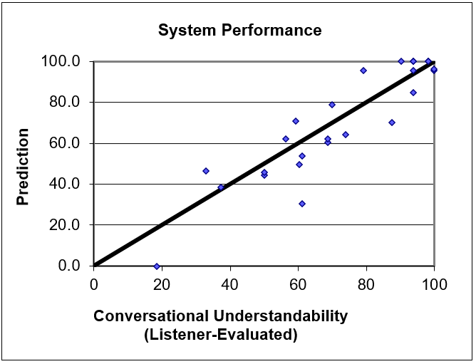
The very first production version of the test needed training on only 25 speakers in all. Because of the knowledge-based foundation, the result performed very well – and not only on the training data (92% correlation: see the figure), nor only on other speakers of the three original L1’s, but then on other, very different ones as well: Ukrainian, Pashtun, and Arabic, among others.
Why could such a small and narrow training set handle such breadth of L1’s? Because the rules for the physics and physiology of speech, and the knowledge of our expert, embody tens or even hundreds of thousands of measurements packaged into a concise framework.
Industry: Remote Sensing Solution:
Solution: Acoustic Modeling and Analysis
A company was interested in how a “listening” system can determine the directions of multiple sound sources from multiple microphones. We implemented an algorithm to detect coincidences of energy at many frequencies, between any pair of microphones.
At any frequency, the peaks of a pure-tone sound wave at one microphone are coincident with peaks at the same time (or phase) in the other if the microphones are separated by any whole number K of wavelengths along the wave’s path. For any K, there is a corresponding direction of the sound wave. With many possibilities open for the correct K, there are many possibilities for the direction. This is what makes pure-tone sources so hard to localize with our ears.
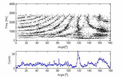
Two sound recordings were played through loudspeakers 1 meter (3′) and recorded by two microphones 0.7 meter (2′) apart. (The samples have little energy above 3 kHz.) One source lay nearly in the “endfire” direction, near 180 degrees, the other at 63 degrees off the axis. The sum of coincidence detections (bottom) over all frequencies shows a clear, narrow peak near 117 degrees (180-63) and a broad peak near 165 degrees. The frequency analysis (top) shows a striking visual pattern for both detections across a range of frequencies and angles, enabling us first to construct a filter matched to this type of pattern and then to use it to detect the directions even more precisely.
Most sound sources, however, produce time-varying energy at many frequencies. By watching for the few directions that are possibilities for many frequencies at once, and by building up the information over time, the system can begin to determine the directions of sources, even of multiple sources present at the same time.
In practice, typical sources come in such a variety that the algorithm produces many false alarms until it has a very large amount of data. We therefore implemented a matched filter for the coincidence pattern that it produces, in order to suppress most of the false alarms while retaining the true detections.
Industry: Pharmaceuticals
Solution: Spectral Analysis
A Fortune-50 company came to us asking three questions about automatic inspection of pharmaceutical compounds:
- How many wavelengths will be needed to distinguish among the spectra of mixtures of the compounds in one second;
- How small a cross-contamination can be detected among the mixtures at this speed; and
- How can these answers be re-determined when the company changes the mixtures, as it does periodically?
We knew that, in order to avoid “cooking” the compounds, the light source could not be intense enough to collect high-precision data in one second. Instead, a spectral scanner would need to use a limited number of wavelengths, or even broad spectral bands, provided they could sufficiently distinguish the spectra. This classic application of principal components analysis (PCA) allowed us to specify the optimal wavelengths for the designers of the light source. Moreover, the answer was based on the compounds themselves, and did not depend on how they would be mixed. For these wavelengths, and with the knowledge of the spectral technology and the time available for inspection, we knew the signal/noise ratio that the device could achieve, which told us immediately how detectable any contamination could be.